MIT 6.824: Lecture 15 - Spark
· 5 min readIn the first lecture of this series, I wrote about MapReduce as a distributed computation framework. MapReduce partitions the input data across worker nodes, which process data in two stages: map and reduce.
While MapReduce was innovative, it came with some limitations:
-
Running iterative operations like PageRank in MapReduce involves chaining multiple MapReduce jobs together. Since a MapReduce job writes its output to disk, these sequential operations require a high disk I/O and have high latency.
-
Similarly, interactive queries where a user runs multiple ad-hoc queries on the same subset of data need to fetch data from the disk for each query.
-
MapReduce's API is restricted. Programmers must represent each computation task as a map-reduce operation.
In essence, MapReduce is inefficient for applications that reuse intermediate results across multiple computations. Researchers at UC Berkeley invented Spark as a more efficient framework for executing such applications. It deals with these limitations by:
-
Caching intermediate data in the main memory to reduce disk I/O.
-
Generalizing the MapReduce model into a more flexible model with support for more operations than just map and reduce.
Table of Contents
Resilient Distributed Datasets (RDDs) #
At the heart of Spark is the Resilient Distributed Datasets (RDDs) abstraction. RDDs enable programmers to perform in-memory computations on large clusters in a fault-tolerant manner. Quoting the original paper:
RDDs are fault-tolerant, parallel data structures that let users explicitly persist intermediate results in memory, control their partitioning to optimize data placement, and manipulate them using a rich set of operators.
We can create RDDs from operations on either data on disk or other RDDs. These operations on other RDDs are called transformations. Examples of transformations are map, filter, and join.
Instead of holding the materialized data in memory, an RDD keeps track of all the transformations that have led to its current state, i.e. how the RDD was derived from other datasets. These transformations are called a lineage. By tracking the lineage of RDDs, we save memory and can reconstruct an RDD after a failure.
There's another class of operations in Spark called actions. Until we call an action, invoking transformations in Spark only creates the lineage graph. Actions are what cause the computation to execute. Examples of actions are count and collect.
Let's look at the following example of a Spark program from the paper.
  lines = spark.textFile("hdfs://...")
  errors = lines.filter(_.startsWith("ERROR"))
  errors.cache()
On line 1, we create an RDD backed by a file in HDFS while line 2 derives a filtered RDD from it. Line 3 asks that the program stores the filtered RDD in memory for reuse across computations.
We can then perform further transformations on the RDD and use their results as shown below.
  // Count errors mentioning MySQL:
  errors.filter(_.contains("MySQL")).count()

  // Return the time fields of errors mentioning HDFS as an array
  // (assuming time is field number 3 in a tab-separated format):
  errors.filter(_.contains("HDFS"))
        .map(_.split(’\t’)(3))
        .collect()
It is only after the first action— count—runs that Spark will execute the previous operations and store the partitions of the errors RDD in memory. Note that the first RDD, lines, is not loaded into RAM. This helps to save space as the error messages that we need may only be a small fraction of the data.
Figure 1 below shows the lineage graph for the RDDs in our third query.
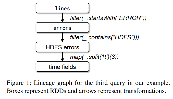
In the query, we started with errors, which is an RDD based on a filter of lines. We then applied two further transformations, filter and map, to yield our final RDD. If we lose any of the partitions of errors, Spark can rebuild it by applying a filter on only the corresponding partitions of lines.
This is already more efficient than MapReduce as Spark forwards data directly from one transformation to the next and can reuse intermediate data without involving the disk.
Note that users can control how the programs stores RDDs. We can choose whether we want an RDD to use in-memory storage or persist it to disk. We can also specify that an RDD's elements should be partitioned across machines based on a key in each record.
Spark Programming Interface #
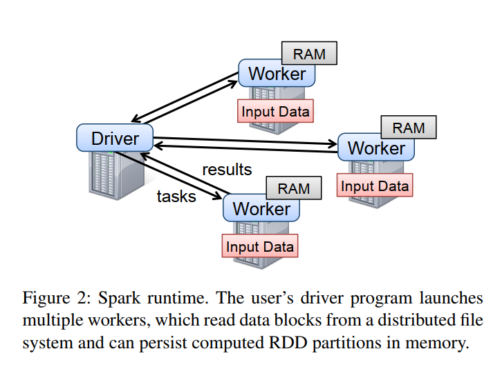
Spark code, as shown in the previous example, runs in a driver machine which manages the execution and data flow to worker machines. The driver defines the RDDs, invokes actions on them, and tracks their lineage. The worker machines store RDD partitions in the RAM across operations. The figure below illustrates this.
Spark supports a wide range of operations on RDDs. You can find a full list of that here.
Representing RDDs #
The Spark implementation represents an RDD through an interface that exposes five pieces of information:
- A set of partitions, which are atomic chunks of the dataset.
- Data placement of the RDD.
- A set of dependencies on parent RDDs.
- A function for computing the dataset based on its parents.
- Metadata about its partitioning scheme.
The table below describes these pieces.
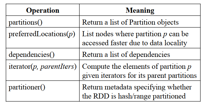
Table 1 - Interface used to represent RDDs in Spark.
The paper classifies dependencies into two types: narrow and wide dependencies. A parent RDD and a child RDD have a narrow dependency between them if at most one partition of the child RDD uses each partition of the parent RDD. For example, the result of a map operation on a parent RDD is a child RDD with the same partitions as the parent.
But with wide dependencies, multiple child partitions may depend on a single partition of a parent RDD. An example of this is in a groupByKey operation, which needs to look at data from all the partitions in the parent RDD since we must consider all the records for a key.
The paper explains the reasons for this distinction:
First, narrow dependencies allow for pipelined execution on one cluster node, which can compute all the parent partitions. For example, one can apply a map followed by a filter on an element-by-element basis. In contrast, wide dependencies require data from all parent partitions to be available and to be shuffled across the nodes using a MapReducelike operation.
Second, recovery after a node failure is more efficient with a narrow dependency, as only the lost parent partitions need to be recomputed, and they can be recomputed in parallel on different nodes. In contrast, in a lineage graph with wide dependencies, a single failed node might cause the loss of some partition from all the ancestors of an RDD, requiring a complete re-execution.
Fault Tolerance #
When a machine crashes, we lose its memory and computation state. The Spark driver then re-runs the transformations on the crashed machine's partitions on other machines. For narrow dependencies, the driver only needs to re-execute lost partitions.
With wide dependencies, since recomputing a failed partition requires information from all the partitions, we need to re-execute all the partitions from start—even the ones that didn't fail. Spark supports checkpoints to HDFS to speed up this process. By doing this, the driver only needs the recompute along the lineage from the latest checkpoint.
Conclusion #
In the evaluation performed by the paper's authors, Spark performed up to 20x faster than Hadoop for iterative applications and sped up a real-world data analytics report by 40x. But Spark isn't perfect. For one, RAM is expensive, and our computation may require a huge RAM for processing in-memory. You can learn about other limitations here.
Overall, Spark's reuse of data in-memory and its wider set of operations make it an improvement over MapReduce for expressivity and performance.
Further reading #
- Resilient Distributed Datasets: A Fault-Tolerant Abstraction for In-Memory Cluster Computing - Original paper from UC Berkeley.
- Lecture 15: Spark - MIT 6.824 lecture notes.
- Spark API Documentation.